
So how do you benchmark biology?

This is a human-readable summary of the EFFECT paper [1]. I found that the process of scientific writing (especially with multiple authors and review rounds) makes texts significantly harder to read than intended - hence this post.
Good benchmarking is a cornerstone of progress in all fields of AI.
The whole premise of AI is being able to figure out hidden connections within your data. However - exactly because these connections are hidden - what the AI actually latches onto may not be what you like.
Benchmarking tanks
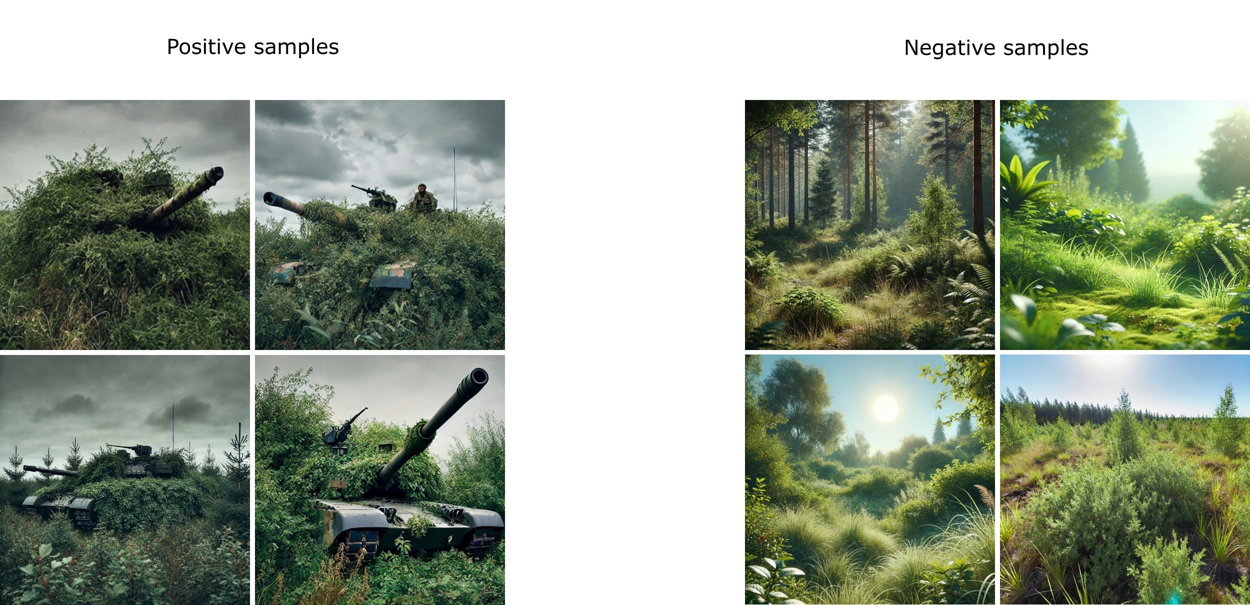
There is an urban legend floating in the AI community about a team who tried to train an AI to recognize tanks. The system worked perfectly on the test benchmarks then immediately failed miserably in the field.
Here’s a set of training images. Guess what happened.
.
.
.
.
The clouds cleared after the tank photos were made, so all negative images were made in sunshine.
So all the AI learned was that no sun = tank, sun = no tank.
But back to biology.
Benchmarking biology
All of this is made exponentially harder by the fact that in biology, we don’t even really have a ground truth to work with. There are tons of unknown, uncontrolled variables in any experiment, and data gets more noisy the deeper you go.
What’s the actual information content of an RNASeq experiment? Which RNA values are trustworthy? How trustworthy they are? Hard to say.
But we need to start somewhere. Let’s try establishing a beachhead and building from there. Let’s start from the most controlled setup possible: secondary, cultured cell lines. Let’s take the metric that’s closest to some form of ground truth: cell viability. Do the cells survive or die in response to your intervention (a drug or a gene knockout, for example)?
This is probably the least noisy information we have, and it even has a particular application in oncology, where you actually want to kill a certain population of cells, but only those cells if possible.
There are two gold standard datasets for this kind of setup: Depmap[2] (for gene knockouts) and GDSC2[3] (for drug effects).
OK, fine. So let’s take Depmap or GDSC2, remove say 20% of the data randomly, and if I can predict the missing data well enough, my method works, right?
Your method will work wonderfully. You will get ~90% accuracy. A lot of people tend to think that viability prediction is a solved challenge in computational biology, we can get methods to be as precise as experimental replicates.
Unfortunately, we were collectively doing the tank thing.
Three things to change
We have found three problems:
1. Most of the data is not surprising. You want to predict the outliers.
Check this sample plot. This is how the data really looks:

Some drugs are just generally stronger than others. Some cell lines are just generally more frail than others.
What’s really useful if you can find the outliers. Is there a mighty resistant cell line which is surprisingly sensitive to your drug? Is there a cell line in which a gene is suddenly essential?
To focus your metrics on the important question don’t use (uncorrected) global correlations1. Calculate a separate correlation value per gene (or per cell) and median-aggregate them. Pearson is better then Spearman as you want to emphasize the outliers. This is similar to what z-score does.
2. We were not splitting to answer the right question.
In how many real situations is both the cell line and the drug of interest known? I’m either giving you a new drug which has not been tested before or want to understand how my drug would fare in patient - who are actually a new environment each.
So either leave some cell lines entirely out of training (we call this a CEX split - cell-line exclusive) or leave entire drugs out (DEX - drug-exclusive).
Now when you leave drugs out, be careful that the drugs you left in are different enough. Some drugs are actually pretty similar to each other so you may inadvertedly leak data. Targeting the same pathway is fine. Depending on your use-case, having some shared protein targets could be OK as long as there’s not too much overlap. This needs some work, but we have some curated splits you can use below2.
There are many other ways to split the data if you have more complex data. Two others we tend to use frequently:
Can you predict a drug’s effect in vivo only from in vitro data? So your drug of interest can only have in vitro data in training, but you can have some other drugs with in vivo data so you understand the environment. We call this PDX-exclusive, as we usually do this when predicting to patient-derived xenograft models implanted in mice.
If given combination data to work with: could you have predicted this combination effect using mono data only for the two drugs in question? Single drugs are easy to test on many cell lines (with a PRISM screen for example), but the cost explodes when you want to test all possible combinations, so in silico is also useful here.
3. There can be more sources of bias present simultaneously.
Many years ago, with some of our first models, we were very happy with our performance. We used z-scores, we did drug-exclusive splits and have gotten surprisingly high scores. Sadly, it was a mirage.
The problem was the general sensitivity of cell lines to drugs [4], as both the split and the metric were only adjusting for drugs.
Under the hood, train/test splitting adjusts for one kind of bias, and a good metric can also adjust for one., However, in this setup the two biases we adjusted for happened to coincide, and cell line bias was left in. You can also easily have more than two sources of bias which you just cannot remove just by combining metrics and splitting.
We needed a more powerful tool.
It’s impossible to programmatically correct for unknown sources of bias, but it is possible to correct for any number of known sources.
We called this tool (creative, I know) the Bias Detector. Just these three steps:
Take a bias prediction from each bias source you want to filter(the mean of all the samples in the training set from the same source, eg. how strong your drug is on average on all of the cell lines in the train set)
Combine all these bias predictions into one bias predictor with a linear model
Your corrected metric is the partial correlation of your prediction and the ground truth with the bias prediction as the controlling variable.
This works with most continuous metrics. It is possible to build a version of the Bias Detector for a classifier based on the same considerations, but it will be slightly less intuitive3.
Solving for viability
The mean partial correlation among drug replicas in GDSC2 is 0.51, so that’s how good we can theoretically be.
How did standard ML algorithms fare after correction? Not well:

Even viability is clearly still unsolved. Which means that it might make sense to ask all the fancy biology foundational models this simple question first: Can it tell us whether the cell would live or die better than a Random Forest?
Only after this would it probably make sense to focus on getting the actual RNA levels right.
RNA prediction does give additional biological insights, but it is also a whole new can of worms. That’s because you don’t just have to fit a single number anymore, but a whole twenty thousand of them. How to balance each? Maybe I could cover some of this in a next post.
We have made a reference benchmark set and our Bias Detector implementation freely available. Do try it if you have something, maybe you finally figured it all out.
Bias Detector code: https://github.com/turbine-ai/DrugKOPred-benchmark-bias
Reference benchmark: https://benchmark.turbine.ai
Thank you Bence Szalai, Imre Gáspár, Valér Kaszás, László Mérő, Milán Sztilkovics for working on this together.
Thanks to Andreas Bender, Aviad Tsherniak, and Daniel Veres for proof-reading the paper and suggesting how to make it more understandable.
References:
[1]: Szalai et al. “The EFFECT benchmark suite: measuring cancer sensitivity prediction performance - without the bias”
[2]: Tsherniak et al. “Defining a Cancer Dependency Map”
[3]: Iorio et al. “A Landscape of Pharmacogenomic Interactions in Cancer”
[4]: Geeleher et al. “Cancer biomarker discovery is improved by accounting for variability in general levels of drug sensitivity in pre-clinical models”
Global correlations corrected for bias are perfectly usable.


The plots above show the performance of standard ML methods measured by bias-corrected global Pearson correlation. As more cell line and drug features are introduced, the performance logically improves (only by adding cell features in the cell-exclusive (CEX) and only by adding drug features in the drug-exclusive (DEX) setup)
The drug splits you can find at https://benchmark.turbine.ai also have some drug targets overlapping between the train and test set, but we took care so that drugs in the test set have at least somewhat different target profiles from any drug in the train set.
What you can do is take a cellwise or drugwise metric, and compare with an appropriate statistical test whether your performance is significantly better than the bias. You can then tally the # of drugs or cells together where you are significantly over bias for a global performance score. What this does not tell you as a global score is how much better are you than the bias on the average drug / cell line.