
Assessing a Virtual Cell’s utility

Hitting 2026 running, I can tell you that the team was asked a lot internally to evaluate and share their opinion on many published approaches on creating virtual cells.
Gerold Csendes was inspired to write down the process he developed for those evaluations.
I converted it into Substack’s format, but had to cut the last chapter due to length limitations. You can get the full PDF here. Gerold, the floor is yours:
We assume the reader has some familiarity with Virtual Cells. For readers new to the field, we advise starting with our blogpost.
The claim is defined by the test data
Genetic perturbations
Chemical perturbations
Can the score measure the claim?
Example 1: Evaluating differential effects in raw expression space
Example 2: Correlation (alone) in wide screens
Summary: Where is the field right now? (only in the PDF)
Intro
Virtual Cells are one of the hottest topics in computational biology right now. The field is chasing an “AlphaFold moment”: a model that turns messy biology into reliable perturbation predictions, at scale. That ambition is worth pursuing, but a sober reality check arrived in early 2025. Multiple groups—including Ahlmann-Eltze et al. and us—showed that several “foundation model” claims on drug discovery benchmarks could be matched or beaten by simple, classical baselines. Since then, new methods have continued to appear, and headline performance on popular benchmarks has often improved.
This note is a practical, drug discovery-facing guide to interpreting such Virtual Cell results. Concretely, we offer a lightweight review checklist that helps you (1) scope what a benchmark result can legitimately claim, and (2) validate whether the evidence is trustworthy.
In this note, we use a narrower definition of Virtual Cells: models that predict perturbation outcomes—e.g., the effect of CRISPRi or a drug on a cellular phenotype (most commonly post-perturbation gene expression). Most widely used Virtual Cell benchmarks follow this framing.
From the outside, it’s tempting to accept a straightforward narrative: Virtual Cells could approach experimental performance, the gap is “just” scaling data, model size, and compute until we get the equivalent of AlphaFold for perturbations. We (Turbine) are building Virtual Cells because we believe this will indeed eventually happen. Still, we think important context is often left out when people assess “utility” from benchmark tables alone. Drug discovery is expensive and failure-prone, and most proof points don’t survive the next step after a leaderboard read.
Our day-to-day work forces that disciplined downstream focus. We constantly benchmark state-of-the-art models, try to separate real progress from evaluation artifacts, and make the case to partners that our model is worth using instead of an open-source alternative. In practice, we found ourselves repeatedly applying a two-stage process: (1) specifying the claim and (2) validating the evidence.
What we generally find is that we are still far from the ambitious definition of Virtual Cells: models that generalize across cell types, perturbation modalities, and datasets. We also find that “validating the evidence” is not straightforward—one needs to read result tables through a critical lens.
The goal of this note is to provide a practical reading guide for benchmark-based claims: first, define what a reported score legitimately implies; second, identify failure modes—such as leakage, weak baselines, or misaligned metrics—that can overstate progress.
Step 1. Specify the claim
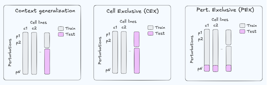
It is not always easy to parse what a method is claiming to do – that is, in what kind of downstream applications would the presented results be applicable. This is often fine in research; authors don’t always need to precisely describe in which context method X can be used. However, if we are talking about Virtual Cell utility, we need to translate that into a claim about usability. Terms like context generalization, out-of-distribution, or capturing cellular behavior frequently appear, but they are hard to validate unless they are grounded in a specific benchmark and split strategy.
The claim is defined by the test data
The most important factor for specifying the claim of a Virtual Cell is the benchmark(s) it is evaluated on. Another central axis is the dataset split strategy, which has a large impact on what conclusions are justified. Today, two benchmark families are especially common in the Virtual Cell space: Perturb-seq CRISPRi genetic benchmarks and the Tahoe-100M drug perturbation benchmark.
Genetic perturbations
Accurate modeling of genetic perturbations is a core challenge for drug discovery. If successful, it could support target identification by narrowing the hypothesis space and generating testable, context-specific predictions (e.g., expected pathway shifts or compensatory programs after target knockdown). Today’s most widely used datasets are Perturb-seq CRISPRi screens measured by post-perturbation transcriptomics, typically spanning only a handful of cell contexts and a perturbation set of essential genes. 1
Because the data are limited, benchmarks often use a gene-exclusive split (GEX, Fig. 1. right) —holding out genes at test time while evaluating in the same cell contexts. This setup has two practical limitations. First, for Target ID, we usually care about predictions in the disease-relevant cellular context (and about selectivity across contexts), whereas GEX evaluates generalization across genes within a small, fixed set of cell types. Second, restricting perturbations largely to essential genes can make the task systematically easier: essential-gene knockdowns often induce stronger and more stereotyped transcriptional programs, which can inflate aggregate metrics without guaranteeing robustness to more diverse, weaker, or more selective perturbations (e.g., non-essential targets, selectivity).
Zooming out, GEX is an artificial holdout from an application standpoint—targets are not “unseen genes” in deployment as much as they are new contexts (new disease state, new genetic background, new cell type). For that reason, strong GEX performance is best interpreted as a diagnostic (does the model properly represent genetic perturbations) rather than as sufficient evidence for Target ID utility.
A more practically useful evaluation is cell-exclusive generalization (CEX, Fig. 1. mid.)—holding out cellular contexts and asking whether a model can predict how the same perturbation behaves across cell types, including selectivity patterns. Unfortunately, CEX is underrepresented in current Perturb-seq benchmarks, making it difficult to test stronger claims about real-world Target ID workflows.
Ultimately, causal understanding of drug and biomarker interactions would necessitate being able to generalize to combinatorial perturbations, with at least one of the perturbations being unseen. This is the setup we most frequently encounter in pharmaceutical applications. The scarcity of public dual-perturbation data means that open-source, large-scale benchmarking of this capability is still unsolved.
Currently the most practical proxy for combinatorial benchmarking would be larger perturbational transcriptomics resources—datasets closer to “DepMap-scale” breadth in cell contexts, but with post-perturbation readouts.
In the near term, the community could adapt more realistic benchmarks by leaning on already available genome-wide Perturb-seq datasets (X-Atlas/Orion2, Replogle et al. K5623) and adopting split protocols that explicitly measure cross-context generalization.
Chemical perturbations
Tahoe-100M is a popular drug perturbation benchmark containing ~50 cell lines and ~1100 compounds. Compared to GDSC, Tahoe-100M is more extensive on the compound axis (1100 vs ~300) but more limited in cellular context (50 vs ~1000 cell lines). It is commonly evaluated with a “context generalization” split, often corresponding to few-shot generalization along an axis (Fig. 1. left). How relevant is this setup for drug discovery decisions? We argue that few-shot generalization can mimic some workflows, but in many settings a fully exclusive setup is more broadly applicable: either drug-exclusive (DEX; Fig. 1. right) or cell-exclusive (CEX; Fig. 1. mid). Data is often scarce, and assuming that the compound in question has little-to-no assay data is a robust default that covers a broader range of applications. For this reason, we propose more challenging and clearly defined Tahoe-100M split protocols (CEX/DEX)
Under current splits, strong results support split-limited claims. Currently, high Perturb-seq performance is a diagnostic tool that clears the model for more specific downstream tests. High Tahoe-100M performance (in the usual context generalization setup, see below) mainly justifies few-shot screening claims. Strong performance on stricter CEX/DEX splits would support broader, more ambitious claims.
Step 2. Validate the evidence
Up until now we have discussed how we can specify a Virtual Cell’s claim given the benchmark it uses. But knowing what a result could claim is only half the story: we also need to decide whether the reported gains are trustworthy and would survive outside the benchmark setting. Reading the results table alone is rarely enough. Below are three questions we find imperative to ask when validating the evidence.
Check for data leakage
Before interpreting any results table, the first question is whether the reported score reflects generalization or memorization. Leakage—when evaluation information sneaks into training—directly undermines trust in benchmark performance.
Leakage is especially easy to introduce when models and data pipelines become complex, and it is a well-known concern in LLM evaluation: models can look strong on public benchmarks yet fail on genuinely new test sets when the data is truly unseen (see Math Olympiad). Similar dynamics appear in biology: when benchmarks contain near-duplicates (e.g., high sequence similarity across train/test) or share structure with training corpora, sophisticated models can appear to win by learning shortcuts rather than transferable biology.
There is a cautionary tale for leakage and benchmarks in the binding affinity benchmarking community. There, the commonly used PDBBind 2020 dataset contained very large, sometimes even 100%, sequence similarity to evaluation sequences (Fig. 4, paper).
Virtual Cells are particularly vulnerable to this risk because many are foundation models pretrained on vast, heterogeneous datasets. If downstream benchmarks (or close variants of them) make their way into pretraining, it becomes difficult to disentangle genuine generalization from memorization. This risk will likely grow as pretraining corpora expand and becomes harder to audit.
Leakage can also be subtle and “context-dependent.” Examples include:
Using proprietary data from the same perturbation domain as model features while reporting performance on an open benchmark.
Constructing perturbation graphs or neighborhood features using information that is only available because the benchmark perturbations are known in advance.
Number of cells per perturbation in single-cell datasets which usually correlates with the strength of the perturbation (VCC was affected, see Fig. 1 here)
These are not necessarily data leaks if the benchmark setup is careful enough—but in most evaluation settings they effectively are, and they should be disclosed and justified.
One practical way to mitigate leakage is evaluation on held-out, non-public test sets, where the training data and benchmark are separated by design. This is why community competitions (e.g., CASP/DREAM-style) are so valuable for measuring “in-the-wild” performance. The Virtual Cell Challenge (VCC) was an important step in that direction for the new era of Virtual Cells, even if the first iteration was largely about learning how to benchmark these new models.
Are the baselines strong and domain-informed?
Benchmarking complex models only against other complex models—especially if the benchmark itself is new—is risky. It can ignore substantial prior work in the domain and makes it hard to contextualize task difficulty. In much of modern AI, the “moment” progress happens is clear: a new architecture must beat strong incumbents (e.g., ViTs on ImageNet). Virtual Cells are not in that regime yet. We do not have a single, widely accepted “ImageNet for perturbations” and neither have we reached a point where a single model family cleanly dominates across settings.
What we do have are decades of biological and experimental insights about how cells, perturbations, and readouts should be represented. These insights already lead to surprisingly strong baselines, and they remain relevant even as model scale increases.
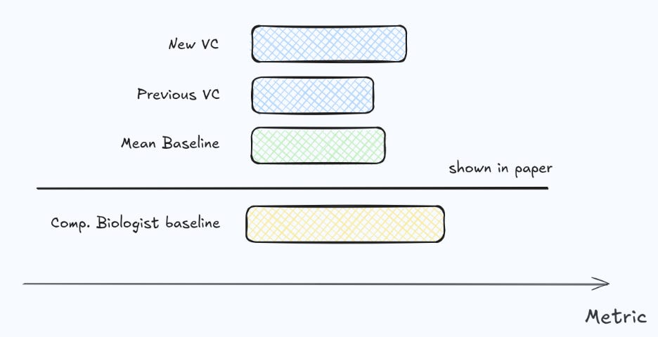
For that reason, we believe a Virtual Cell should be evaluated not only against “mean” and simple linear additive models, but also against a class of stronger, domain-informed methods—what we call computational biologist baselines (what an experienced computational biologist does on first approach trying to predict from the same data - see our random forest or ridge as an example). Concretely, these are models that deliberately encode biological structure (e.g., sensible covariates, perturbation graph structure, batching and control modeling, and cell-context conditioning) without requiring foundation-model scale.
It is encouraging that reporting simple baselines on perturbation benchmarks is becoming standard practice. Still, we often find that baselining is not yet rigorous enough: there is a large space between trivial baselines and the most complex Virtual Cells, and that middle ground is frequently underexplored. In our own evaluations, investing effort into this “computational biologist baseline” space often closes much of the apparent gap to SOTA—and not so rarely matches or outperforms it—changing the conclusion about whether a complex Virtual Cell is worth deploying.
Can the score measure the claim?
A strong benchmark score does not automatically mean a Virtual Cell is making useful predictions. In post-perturbation transcriptomics it is possible to achieve impressive-looking metrics while missing what matters in practice—e.g., capturing differential response, pathway-level shifts, or clinically meaningful rankings (which compound/target moves the biology in the desired direction). Several recent efforts argue for improved evaluation e.g. Systema, PerturBench, Diversity by Design, STATE but the field is still far from consensus, and community efforts like the Virtual Cell Challenge have highlighted how difficult it is to select a robust metric suite.
Why is this problem so hard? One key difference from protein structure prediction is that structure has a relatively intuitive geometry: predictions can be compared to ground truth in 3D, and “closeness” has a fairly direct interpretation. Post-perturbation transcriptomics, by contrast, is a ~20k-dimensional vector whose biological meaning is largely read out indirectly (e.g., through differential expression, pathway activity, and phenotype proxies). As a result, many “reasonable” metrics end up rewarding the wrong behavior.
This is not to say current metrics are useless, some are informative. But there are common choices that systematically overstate progress. Below are two failure modes we see often.
Example 1: Evaluating differential effects in raw expression space
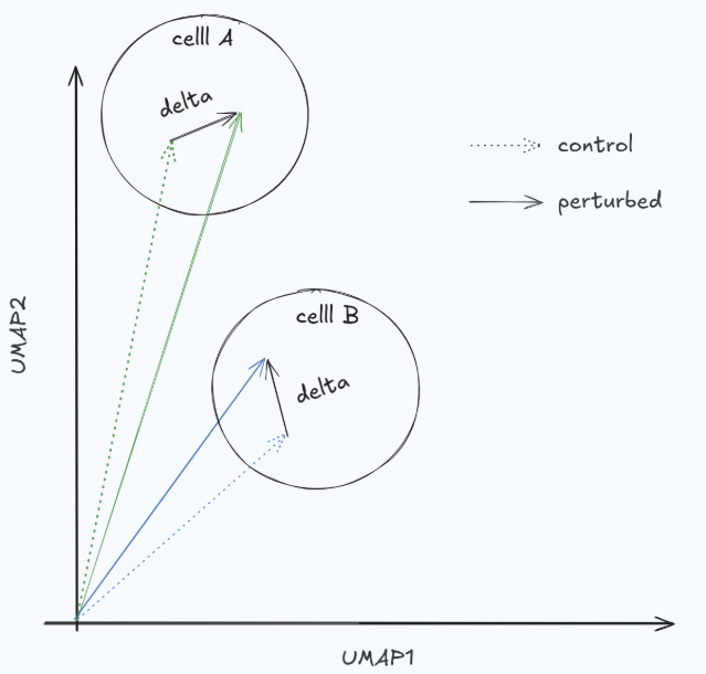
In perturbation studies, what we care about is the differential effect: the change relative to an unperturbed (or matched control) state. Raw expressions mostly reflect cell identity, and in many settings the perturbation effect is comparatively small (Fig. 3). If a metric evaluates predictions in raw expression space, it can reward models for predicting baseline identity rather than perturbation response—artificially inflating scores and encouraging “do nothing” behavior. A simple no-change baseline (predict the control) is a useful sanity check here: if it scores surprisingly well, the metric is likely not measuring the perturbation biology you care about.
Example 2: Correlation (alone) in wide screens
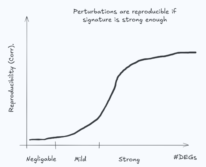
Correlation in differential expression space can be useful—but only when the perturbation induces a reproducible, sufficiently strong signature. If the true effect is near zero, the measured differential expression is dominated by noise and won’t reliably reproduce in the lab (Fig. 4). It is unrealistic (and undesirable) to expect a model to match such examples. This is not a corner case: many genetic perturbations have weak transcriptomic effects, and many drug–cell–dose combinations produce negligible response. In these regimes, correlation becomes unstable and can penalize sensible behavior while rewarding overfitting or noise chasing.
A practical implication: metrics should be effect-size aware (e.g., stratify or weight by signature strength / experimental reproducibility), and evaluation should explicitly distinguish “predicting a real signal” from “predicting noise.”
Is it learning actual biology?
In drug discovery, we don’t just care about a good average prediction—we care about whether a model captures, in a way we can measure and quantify, the causal functional impact of a perturbation on a cell. In practice, this means asking whether the model’s internal representation supports the manipulations we routinely reason with: dose changes, target engagement, pathway relationships, and cross-modality links (genetic vs. chemical perturbations). We treat these as diagnostic checks: passing them does not prove the model is “right,” but failing them is often a warning sign that the model is exploiting shortcuts or missing structure that will matter in real deployments.
We’re cautious with “priors”: scientific history is full of surprises, and some intuitions will be wrong. Still, when a Virtual Cell both performs well and exhibits coherent, controllable behavior under these diagnostics, it is a strong reason to investigate deeper. Conversely, incoherence often points directly to where evaluation, data assumptions, or modeling choices are failing. The Large Perturbation Model is an example of exhibiting patterns of coherent representations.
Without loss of generality, we look for:
Dose response and directionality: does increasing dose move the predicted state consistently (and saturate plausibly), rather than producing erratic jumps?
MoA sensitivity vs chemistry sensitivity: Do drugs with shared mechanism of action cluster more strongly than drugs with superficial chemical similarity? Can the model separate on-target effects from confounders such as general toxicity or stress responses?
Target ↔ pathway consistency: if a pathway is genetically perturbed in training, does the model generalize to drugs acting on that pathway in a predictable way?
Cross-modality alignment: are a single-target inhibitor and its KO/CRISPRi analogue represented as “nearby” in the right contexts? More importantly, does genetic evidence improve out-of-distribution drug predictions in a measurable way?
Attribution sanity: when the model predicts a response, can we attribute it to plausible genes/pathways rather than dataset artifacts (batch, cell line identity proxies, etc.)?
Thanks to Bence Szalai and Krishna Bulusu for reviewing and improving this note.
These are datasets from Replogle el. al and Nadine et. al
Spanning 2 cells: HCT116 and HEK293T
The “pan-expression” wide version
 | A guest post by
|