How did we get a regression model to the top of the Virtual Cell Challenge

and what this tells us about the state of computational biology

This post is a high-level summary of our key learnings. You can find a more detailed and technical write-up on our Challenge experience here: Mean Predictors write-up

It’s been a while since the last DREAM challenge tested our ability to predict cellular responses. ARC took up the mantle with their Virtual Cell Challenge.

Naturally, we joined. We are the meanest predictors, after all.

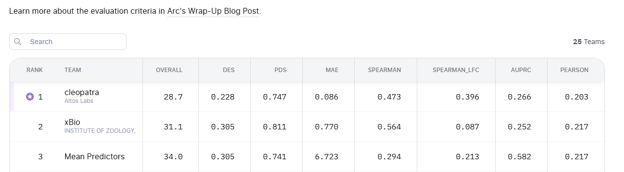
In the end, a simple model first described in 1970 climbed to the top of the leaderboard for a while and ultimately landed 15th overall, and became one of the best “generalist” model under ARC’s newly announced criteria.

The placement itself is not what matters. What’s interesting is why this model was the right choice.

State of the VCC leaderboard at the 14th of October

The newly announced Generalist Leaderboard

Single cells are only useful if they are different

There’s a strong temptation to treat single-cell measurements as “big data.” After all, Perturb-Seq gives you reads from hundreds of thousands of cells. But what you get from each cell is just a somewhat redundant fragment of the biological reality.

In practice, we’ve always found that the information content comes from how many distinct pseudobulks (clusters) you can form. In heterogeneous ex vivo material, you can get 20–50 clusters per condition.

However, in Perturb-Seq, colonies are are relatively homogeneous. The true value of the technology lies in making it possible to do many conditions together in one flask, not in it being single-cell. So the number of effective data points you have is 1 RNASeq data point per condition.

So, as an exercise, how many effective RNASeq data points does Tahoe-100M have?

Based on the description, they multiplex 50 cells with 1100 perturbations - giving an effective data size 55,000 data points.

Which means that in practice, for all the cells sequenced in VCC, the effective dataset looked roughly like this:

• 150 training points

• 50 for the leaderboard

• 100 for the final evaluation

which means 300 effective data points.

This is why many teams like us chose to ignore the individual cells entirely and went to only predict the clusters’ behavior, still finishing in the top spots. I think this is pretty strong evidence that using all the single cells adds little to no additional information despite using magnitudes more compute.

The bottleneck today is data, not AI

If you add up the useful RNASeq-like data available to the field - Perturb-Seq, Tahoe (Drug-Seq), regular RNASeq, even LINCS (Broad’s public microarray-like dataset) - you will get to something like half a million effective datapoints. Compare this to the number of possible configurations of a 20,000-gene system and it becomes clear we still only see the tip of the iceberg. So regularization and inductive bias is still paramount.

Therefore, an AI architecture is only as good as (1) its ability to ingest the limited data we have, and (2) the inductive biases that allow it to exploit symmetry and structure.

So don’t dismiss simple models like regression or Random Forest. Given the same data, they can perform on par with far more complex architectures, and often generalize better to other tasks.

The person I probably learned the most from about machine learning is Prof. Abu-Mostafa. He said that your model should match the complexity of your data, not the complexity of your problem.

In 2025, we can formulate this as a philosophical razor:
The simplest model that covers your data and inductive bias will generalize best.

Relevant data beats more data. Put the work in.

We did not use any pretraining to get this high on the leaderboard. This reinforced our view that, today, foundation models offer little to no added value predicting perturbation effect.

What did matter were the handful of other Perturb-Seq datasets we found (Replogle et al., Nadig et al.) which contributed most of our predictive power¹. These represent a tiny amount of data both compared to pre-training datasets (Geneformer) and to large-scale perturbation screens (LINCS or DepMap), but are much closer to the physical assay we aimed to predict.

However, incorporating these datasets required weeks of cleaning, alignment, and integration. Smaller teams recoiled from this work. We had the experience and tooling to do it, and it made a substantial difference. What matters is putting the work in.

Even a small set of 50–100 data points can materially improve prediction accuracy when those points are closer to the real scenario you aim to model than anything else available.

Metrics are hard, but especially in 20,000 dimensions

Measuring prediction performance in a way that reflects real-world use is notoriously difficult. Models hammer any scoring function thousands of times per GPU-second. If your metric has loopholes, the models will find and exploit them.

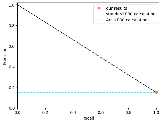
We always generate scatterplots, as strange patterns often reveal metric artifacts. For example, this is how we just discovered that ARC’s AUPRC method was unexpectedly generous to pseudo-bulk predictions².

Now all of this becomes exponentially harder if you are trying to score predictions in a 20,000 dimensional space.

Trying to do all this in 20,000 dimensions amplify these issues. The core VCC metric PDS (Perturbation Discrimination Score) ranks which true perturbation vector your prediction is closest to. But what does “closest” really mean?

Teams quickly learned that the magnitude of the predictions matters more than the direction of the RNA vector, leading to teams scaling transformations to get better (but biologically not necessarily more correct) PDS scores.

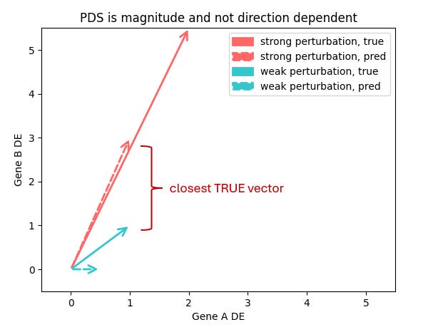
Are you more interested in which genes change, or how much they change? And is a model that gets a subset of genes quantitatively right better than one that gets most genes only qualitatively right?

I don’t think it’s possible to have a single answer to this unless we completely understand how RNA levels map to the internal cell state. Which we don’t.

I don’t think we can clearly resolve this without fully understanding how RNA levels map onto the cell’s internal state - and that’s still ahead of us. Until then, the “right” metric is fundamentally tied to the downstream application you care about.

ARC’s metrics received plenty of criticism, but as general-purpose measures, they are not nearly as flawed as portrayed. They capture different facets of the prediction vector. They can (and should) be hardened, but given the lack of a universal downstream task, VCC’s choices were a reasonable first attempt.

For our applications, we prefer Pearson delta, which tests whether the pattern across the top differentially expressed genes is preserved³.

But don’t forget that RNA-seq prediction itself is not the end goal.

It’s best to evaluate virtual cells at the application

In applied settings, you want to know whether your predictions hold in real life: cell viability, cytokine levels, metabolism, motility - anything tied directly to phenotype. RNA-seq is only a fingerprint of the cell’s internal, unobservable state. And a fingerprint of a proxy will never fully answer the question you care about.

If you want to evaluate virtual cells, measure them at the application layer. That removes the guesswork about whether the model captured the part of the cell state from RNA that matters for your task.

This is not to diminish the value of RNA-seq itself. Post-treatment transcriptomics remains the closest thing we have to a generic, reusable data type - a kind of connective tissue that can link many downstream assays together.

So, do we have Virtual Cells or not?

To some degree. The VCC results show that with relevant data you can approach wet-lab reproducibility for certain perturbation effects.

But the challenge was not difficult enough to demonstrate robust cross-assay generalization, which is a key requirement for truly general virtual cells. Our internal experiments confirm this remains unsolved.

A huge thank you to the meanest predictors: Bence Szalai, Gerold Csendes, Bence Czako and Gema Sanz who did lion’s share of the work.

And of course, thanks to the ARC team for all the work they put in to make this challenge happen! We really enjoyed it.

1. We added the external Perturb-Seq datasets as input features, not as additional training data. That is mostly an implementation detail, but worth noting.

2. How do you draw an AU-PRC curve when you only have a single point? Under the standard trapezoidal rule, you would project that point onto the Y-axis. ARC’s more generous interpretation is that if you push the threshold all the way to zero, you trivially achieve infinite precision.

3. Pearson delta only works when the perturbation produces a sufficiently large effect. Otherwise, you are simply correlating your predictions with experimental noise. You must first filter for responders. The number of data points that survive that filter will probably make you sad.